|
Computational Toolsmiths
Software Tools for Computational Science, Engineering, and Medicine |
FirWav Filter Library
- Summary of the FirWav Filter Library
- Wavelet Filter Bank Standards
- Empirical Tests for Multirate Filter Bank Parameters
- Examples of Individual Filters
- Daubechies Real Biorthogonal Balanced Regular (DRBBR)
- Daubechies Complex Orthogonal Most Symmetric (DCOMS)
- Daubechies Real Orthogonal Least Asymmetric (DROLA)
- Examples of Filter Families
Summary of the FirWav Filter Library
The FirWav Filter Library contains algorithms for numerically computing filter coefficients for the complete set of min-length max-flatness filters that can be derived by spectral factorization of the Daubechies polynomial. It also contains a comprehensive set of routines for the analysis and display of these filters. FirWav filters and algorithms are documented in:
- Taswell, June 1999, Constraint-Selected and Search-Optimized Families of Daubechies Wavelet Filters Computable by Spectral Factorization .
- Taswell, August 1998, Disjoint Sets of Daubechies Polynomial Roots for Generating Wavelet Filters with Extremal Properties .
- Taswell, June 1998, The Systematized Collection of Daubechies Wavelets .
- Taswell, June 1998, Correction for the Sherlock-Monro Algorithm for Generating the Space of Real Orthonormal Wavelets .
- Taswell, May 1998, A Spectral-Factorization Combinatorial-Search Algorithm Unifying the Systematized Collection of Daubechies Wavelets .
- Taswell, April 1998, Numerical Evaluation of Time-Domain Moments and Regularity of Multirate Filter Banks .
- Taswell, March 1998, Empirical Tests for the Evaluation of Multirate Filter Bank Parameters .
- Taswell, December 1997, The Systematized Collection of Wavelet Filters Computable by Spectral Factorization of the Daubechies Polynomial .
- Taswell, September 1997, Computational Algorithms for Daubechies Least Asymmetric, Symmetric, and Most Symmetric Wavelets .
- Taswell, August 1995, Algorithms for the Generation of Daubechies Orthogonal Least Asymmetric Wavelets and the Computation of Their Holder Regularity .
In this systematized collection, the terms symmetric and asymmetric have been used in reference to the actual coefficients, whereas the modifying superlatives least and most have been used in reference to the phase nonlinearity of the coefficients.
The filter design algorithms have been implemented to permit flexible incorporation of other design optimization criterion such as time-frequency uncertainty, frequency-domain selectivity, and time-domain regularity in addition to the phase nonlinearity criterion. Pedagogy has been emphasized in the implementation of the software with plots that display most steps of the design process. Of course, for efficient computation (rather than educational use), these displays can be switched off.
Use of information from this web page should be acknowledged with proper citation. All figures on this page are Copyright © 1997-1999 Carl Taswell and may not be reproduced without the author's permission.
Wavelet Filter Bank Standards
Different definitions and conventions have been used for wavelet filter banks by various authors in their papers, books, and software packages. However, filter bank conventions and algorithm reproducibility standards can be established using clearly specified principles rather than arbitrary choice. Please refer to papers on reproducibility standards downloadable from the Reports Page. Simple examples are provided here regarding choice of norm, parity, and phase for the filter banks. Complete details are available in The Systematized Collection of Daubechies Wavelets .
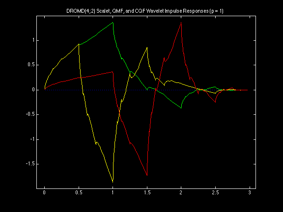
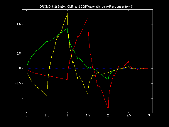
The figures below display estimates of the continous impulse and frequency responses for the scalet (green curve), QMF wavelet (yellow curve), and CQF wavelet (red curve) that can be generated from the the famous compact orthogonal Daubechies wavelet filter coefficients of length 4 and order 2. The splash screen image for WavBox Software displays these wavelets superimposed on top of a characteristic wavelet tiling of the time-frequency plane. FirWav Filter Library commands and MATLAB output follow:
>> K = 2; f = fcdrold(K), g = qmf(f), h = cqf(f)

f =
    0.4830    0.8365    0.2241   -0.1294

g =
    0.4830   -0.8365    0.2241    0.1294

h =
    0.1294    0.2241   -0.8365    0.4830

>> plotwir([f(:),g(:),h(:)])
>> plotwfr([f(:),g(:),h(:)])
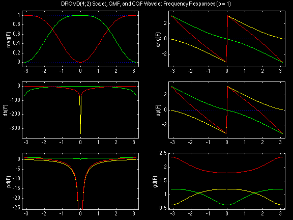
Titles have been added to the plots showing the default value of the parity p = 1. Default norm on these coefficients is coef sum = sqrt(2) and default phase is chosen so that the analysis scalet has minimax group delay. An analogous example with opposite parity p = 0 follows:
>> K = 2; p = 0; f = fcdrold(K), g = qmf(f,p), h = cqf(f,p),

f =
    0.4830    0.8365    0.2241   -0.1294

g =
   -0.4830    0.8365   -0.2241   -0.1294

h =
   -0.1294   -0.2241    0.8365   -0.4830

>> plotwir([f(:),g(:),h(:)])
>> plotwfr([f(:),g(:),h(:)])
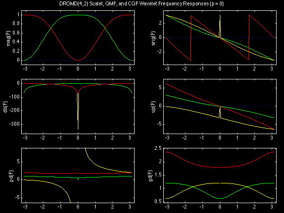
Note that the QMF and CQF wavelets have the same magnitude response but different phase response. An analysis/synthesis filter bank system using a CQF bank yields a perfect reconstructing system whereas one using a QMF bank does not. Here are the analysis and synthesis filter banks for this real orthogonal example (with default parity p = 0):
>> [cA,cS] = cqf(f)

cA =
   4.8296e-01  -1.2941e-01
   8.3652e-01  -2.2414e-01
   2.2414e-01   8.3652e-01
  -1.2941e-01  -4.8296e-01

cS =
  -1.2941e-01  -4.8296e-01
   2.2414e-01   8.3652e-01
   8.3652e-01  -2.2414e-01
   4.8296e-01  -1.2941e-01
For each analysis (cA) and synthesis (cS) filter bank, the lowpass scalet is in the first column, and the highpass wavelet is in the second column. This convention can be demonstrated further with a more detailed example involving complex orthogonal wavelets:
>> K = 4; f = fcdcola(K), g = qmf(f), p = paraconj(f), h = cqf(f)

f =
  Columns 1 through 4
  -0.0178 + 0.0843i   0.1020 + 0.1409i   0.5129 - 0.1398i   0.6822 - 0.3095i
  Columns 5 through 8
   0.2613 + 0.0266i  -0.0829 + 0.1963i  -0.0494 + 0.0289i   0.0058 - 0.0277i

g =
  Columns 1 through 4
  -0.0178 + 0.0843i  -0.1020 - 0.1409i   0.5129 - 0.1398i  -0.6822 + 0.3095i
  Columns 5 through 8
   0.2613 + 0.0266i   0.0829 - 0.1963i  -0.0494 + 0.0289i  -0.0058 + 0.0277i

p =
  Columns 1 through 4
   0.0058 + 0.0277i  -0.0494 - 0.0289i  -0.0829 - 0.1963i   0.2613 - 0.0266i
  Columns 5 through 8
   0.6822 + 0.3095i   0.5129 + 0.1398i   0.1020 - 0.1409i  -0.0178 - 0.0843i

h =
  Columns 1 through 4
  -0.0058 - 0.0277i  -0.0494 - 0.0289i   0.0829 + 0.1963i   0.2613 - 0.0266i
  Columns 5 through 8
  -0.6822 - 0.3095i   0.5129 + 0.1398i  -0.1020 + 0.1409i  -0.0178 - 0.0843i
Note that the CQF wavelet is the paraconjugate of the QMF wavelet. Logical test functions ismbior,
ismorth, and isprfb with truth value outputs for test results are defined
in the tech reports available from the Reports Page. When the QMF and
CQF filters are configured in analysis/synthesis filter bank systems and tested for M-shift biorthogonality,
M-shift orthogonality, and perfect reconstruction, we get the following results for the QMF analysis
and synthesis banks qA and qS, and the CQF analysis and synthesis banks cA and cS.
>> [qA,qS] = qmf(f)

qA =
  -0.0178 + 0.0843i  -0.0178 + 0.0843i
   0.1020 + 0.1409i  -0.1020 - 0.1409i
   0.5129 - 0.1398i   0.5129 - 0.1398i
   0.6822 - 0.3095i  -0.6822 + 0.3095i
   0.2613 + 0.0266i   0.2613 + 0.0266i
  -0.0829 + 0.1963i   0.0829 - 0.1963i
  -0.0494 + 0.0289i  -0.0494 + 0.0289i
   0.0058 - 0.0277i  -0.0058 + 0.0277i

qS =
  -0.0178 + 0.0843i   0.0178 - 0.0843i
   0.1020 + 0.1409i   0.1020 + 0.1409i
   0.5129 - 0.1398i  -0.5129 + 0.1398i
   0.6822 - 0.3095i   0.6822 - 0.3095i
   0.2613 + 0.0266i  -0.2613 - 0.0266i
  -0.0829 + 0.1963i  -0.0829 + 0.1963i
  -0.0494 + 0.0289i   0.0494 - 0.0289i
   0.0058 - 0.0277i   0.0058 - 0.0277i

>> qtv = [ismbior(qA,qS),ismorth(qA),ismorth(qS),isprfb(qA,qS)]

qtv =
     0     0     0     0

>> [cA,cS] = cqf(f)

cA =
  -0.0178 + 0.0843i  -0.0058 - 0.0277i
   0.1020 + 0.1409i  -0.0494 - 0.0289i
   0.5129 - 0.1398i   0.0829 + 0.1963i
   0.6822 - 0.3095i   0.2613 - 0.0266i
   0.2613 + 0.0266i  -0.6822 - 0.3095i
  -0.0829 + 0.1963i   0.5129 + 0.1398i
  -0.0494 + 0.0289i  -0.1020 + 0.1409i
   0.0058 - 0.0277i  -0.0178 - 0.0843i

cS =
   0.0058 + 0.0277i  -0.0178 + 0.0843i
  -0.0494 - 0.0289i  -0.1020 - 0.1409i
  -0.0829 - 0.1963i   0.5129 - 0.1398i
   0.2613 - 0.0266i  -0.6822 + 0.3095i
   0.6822 + 0.3095i   0.2613 + 0.0266i
   0.5129 + 0.1398i   0.0829 - 0.1963i
   0.1020 - 0.1409i  -0.0494 + 0.0289i
  -0.0178 - 0.0843i  -0.0058 + 0.0277i

>> ctv = [ismbior(cA,cS),ismorth(cA),ismorth(cS),isprfb(cA,cS)]

ctv =
     1     1     1     7
In the FirWav functions ismorth and ismbior, the default value for M is 2
for these 2-band filter bank systems. Note that the QMF bank is neither M-shift biorthogonal nor perfect
reconstructing (subject to default error tolerances). However, the CQF bank system is both M-shift
biorthonogal, M-shift orthogonal, as well as perfect reconstructing with a system delay of 7 samples.
The following four figures display the frequency responses for the QMF and CQF analysis and synthesis
banks for this example with the DCOLA(8;4)
wavelets:
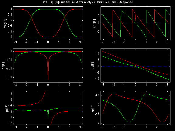

Note that the group delays for the scalet and wavelet cross each other above for the QMF bank, but do not cross each other below for the CQF bank.
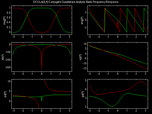
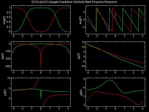
For the CQF bank system above, note that the analysis and synthesis filter banks are configured so that the analysis scalet is chosen to be the one with minimax group delay.
The FirWav Filter Library constitutes only a subset of the more comprehensive WavBox Software Library. Using some additional expert system utilties from the latter, we can generate a more complete report on experimentally observed values of filter bank test parameters for this same example:
>> setwb('FILTYP','dcola','ANAPAR',4); getwb('FBTEST');

FilterBankName = DCOLA(8;4)
FilterBankDelay = 7
FilterBankError = 4.47545e-016
AnaPhaseNonLinearity = 1.95778
SynPhaseNonLinearity = 1.95778
AnaTimeDomRegularity = 1.45266
SynTimeDomRegularity = 1.45266
AnaFreqDomSelectivity
   7.479e-001   7.479e-001
SynFreqDomSelectivity
   7.479e-001   7.479e-001
AnaTimeFreqUncertainty
   8.293e-001   8.293e-001
SynTimeFreqUncertainty
   8.293e-001   8.293e-001
AnaVanishMomentNumber
      0      4
SynVanishMomentNumber
      0      4
Test result values that appear to be duplicated are identical as expected for these orthogonal filters. In the case of biorthogonal filters, the values for analysis and synthesis filters are usually not equal. Note that all values (except the FilterBankName) are experimentally observed values, including the FilterBankDelay and the VanishingMomentsNumber.
Empirical Tests for Multirate Filter Bank Parameters
For complete sets of multi-color figures demonstrating estimation of the filter bank parameters for the DRBBR(10,10;5,5), DCOMS(22;11), and DROLA(26;13) examples below, view the MRFB Parameters Page.
For detailed documentation, refer to:
- Taswell, June 1998, The Systematized Collection of Daubechies Wavelets .
- Taswell, March 1998, Empirical Tests for the Evaluation of Multirate Filter Bank Parameters .
Parameters include:
- Mth-band Interpolation Error mie(f)
- M-band Reconstruction Error mre(A,S)
- M-band Reconstruction Delay mrd(A,S)
- M-shift Biorthogonality Error mbe(A,S)
- M-shift Orthogonality Error moe(F)
- Phase NonLinearity pnl(F)
- Frequency Domain Selectivity fds(F)
- Time Frequency Uncertainty tfu(F)
- Time Domain Regularity tdr(F)
- Time Domain Centers tdc(F)
- Time Domain Moments tdm(F)
- Vanishing Moments Numbers vmn(F)
Examples of Individual Filters
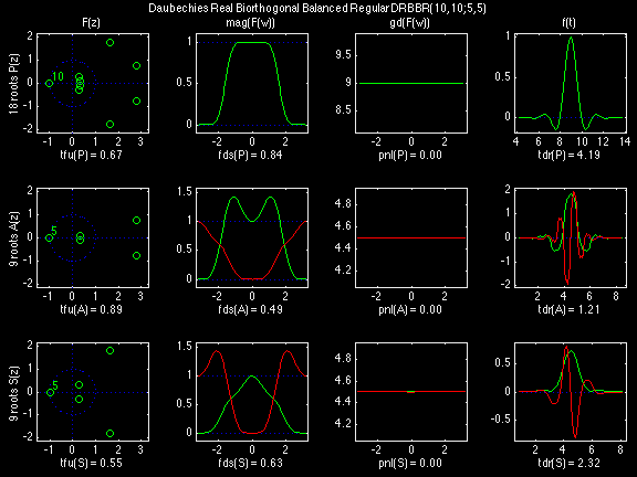
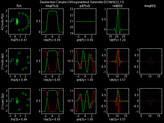
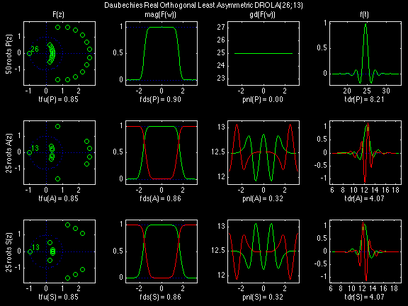
In the following examples of filters, each figure contains a matrix of subplots with rows corresponding to product, analysis, and synthesis filters, and with columns corresponding to characteristics of the filters in the complex Z domain, the frequency domain, and the time domain.
In addition to the abbreviations for the above parameters, figure legend abbreviations for the plots on this page also include:
- f(t) = filter in time t domain
- F(z) = filter in complex z domain
- F(w) = filter in frequency w domain
- mag(F) = magnitude of F(w)
- db(F) = magnitude of F(w) in decibels
- ang(F) = phase angle of F(w)
- up(F) = unwrapped phase angle of F(w)
- pd(F) = phase delay of F(w)
- gd(F) = group delay of F(w)
- P(z) = Product filter
- A(z) = Analysis filter, primary spectral factor of P(z)
- S(z) = Synthesis filter, complementary spectral factor of P(z)
Scalets (lowpass filters) are in green; wavelets (highpass filters) are in red. In the z domain plots, the number near the zero at z = -1 indicates the multiplicity of that zero. This number determines the theoretical number of vanishing moments of the corresponding wavelet filter.
Daubechies Real Biorthogonal Balanced Regular (DRBBR)
This example, DRBBR(10,10;5,5), is the shortest in this family defined by maximizing the balanced time-domain regularity subject to constraint of equal length filters and equal numbers of vanishing moments on both analysis and synthesis filters.
Daubechies Complex Orthogonal Most-Symmetric (DCOMS)
This example, DCOMS(22;11), demonstrates that the complex filters of this family have nonlinear phase despite their symmetric coefficients. However, only the scalets are symmetric, while the wavelets are anti-symmetric. DCOMS(22;11) is the shortest in this family with pnl(F)<=1.
Daubechies Real Orthogonal Least-Asymmetric (DROLA)
Of all filters with <=40 coefficients in this family, this example, DROLA(26;13), has the smallest value <1 for phase nonlinearity yet it also has a value >4 for time-domain regularity.
Examples of Filter Families
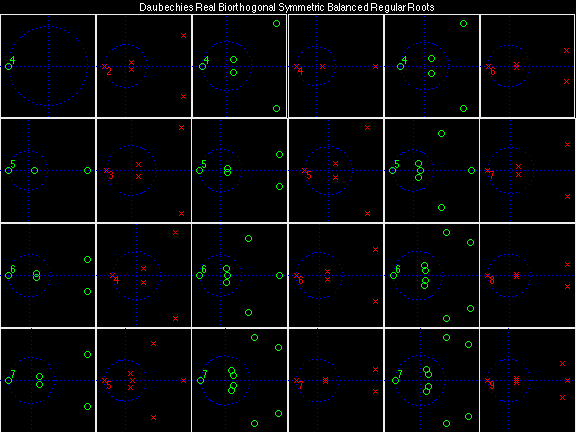
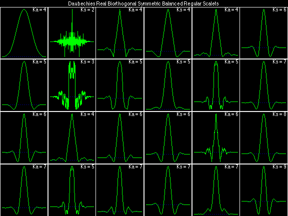
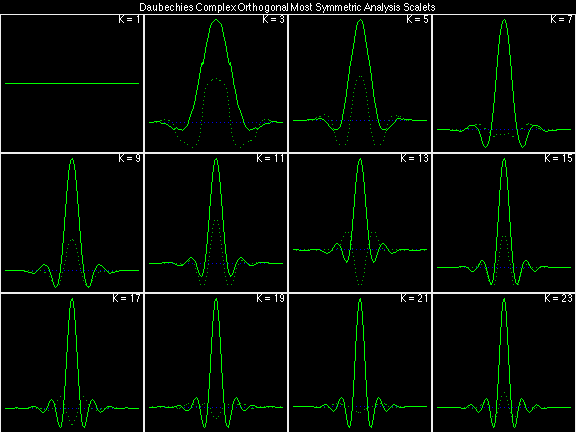
The filter families displayed below
- Daubechies Real Biorthogonal Balanced Regular
- Daubechies Complex Orthogonal Most Symmetric
- Daubechies Real Orthogonal Least Asymmetric
correspond to the examples of the individual filters DRBBR(10,10;5,5), DCOMS(22;11), and DROLA(26;13) displayed above on this web page. In addition to these examples, all FirWav filter families in this collection including the various
families are catalogued on separate web pages. For more detailed notes, refer to these separate web pages.
Daubechies Real Biorthogonal Balanced Regular (DRBBR)

Daubechies Complex Orthogonal Most Symmetric (DCOMS)


Daubechies Real Orthogonal Least Asymmetric (DROLA)
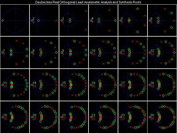
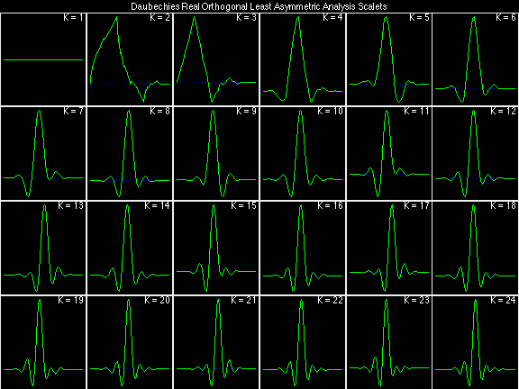
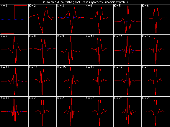
Note that families defined by each of the various defining criteria are not necessarily unique for all K in each family. In other words, for a given K, the wavelet defined by a certain criterion for one family may be the same as the wavelet defined by another criterion for another family. However, even if true for one value of K for two different families, it is not necessarily true for all values of K for those two families.